matlab_learning

(xticklabel, yticklabel, latex): an example
latex interpreter
maximize figure
legend items organization
legend: multiple lines in one legend item
legend: multiple legend boxes
legend: dense data with sparse marker
legend: dense data with sparse marker
legend(ah,p(3:4)) ??
legend: columnlegend.m
legend: gridLegend.m
manipulate figure positions
returns of legend, figure, axis, axes, etc
gcf, gca, etc
errorbar
save data
save in eps, pdf, jpg formats (print)
read & write
rgn setting
diary
fopen, fclose
set path, startup path
eval, mkdir, copy, paste, delete, etc.
make a folder, delete a folder
make a file (with extension), delete a file
mkdir, eval
fopen, fclose, fwrite
text
small figure in big: example 1
small figure in big: example 2
make a vedio
groot: Graphics root object - MATLAB groot - MathWorks (starting from 2014b)
delete white margin
done

%{
This html is generated by the following codes:
    opts = [];
    opts.outputDir = 'matlab_tricks';
    opts.format = 'html';
    publish('matlab_learning.m',opts);
%}

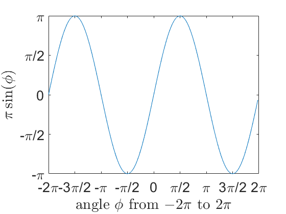
(xticklabel, yticklabel, latex): an example

clear; close all; clc;
x = -2*pi:0.1:2*pi;
plot(x,pi*sin(x));

set(gca, ...
 'xlim',[-2*pi 2*pi], ...
 'xtick',-2*pi:pi/2:2*pi, ...
 'xticklabel',{'-2\pi' '-3\pi/2' '-\pi' '-\pi/2' '0' '\pi/2' '\pi' '3\pi/2' '2\pi'}, ...
 'ylim',[-pi pi], ...
 'ytick',-pi:pi/2:pi, ...
 'yticklabel',{'-\pi' '-\pi/2' '0' '\pi/2' '\pi'}, ...  'fontname','symbol', ...
 'fontsize',20);
% 'Interpreter','latex');

xlabel('angle $\phi$ from $-2\pi$ to $2\pi$','Interpreter','latex');
%     'fontname','helvetica', ... %'fontsize',30);

ylabel('$\pi\sin(\phi)$', 'Interpreter','latex'); %... 'fontname','helvetica');

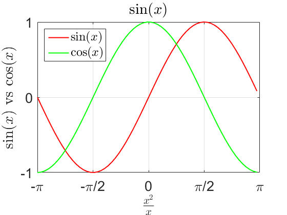
latex interpreter

clear; close all; clc;
lw = 1.5; % linewidth
fs = 20; % fontsize
figure; % axes('fontsize',fs);
x = -pi:0.1:pi;
y1 = sin(x);
y2 = cos(x);
plot(x,y1,'r-', ...
    x,y2,'g-', ...
    'linewidth',lw);
grid on;
set(gca, ...
 'xlim',[-pi pi], ...
 'xtick',-pi:pi/2:pi, ...
 'xticklabel',{'-\pi' '-\pi/2' '0' '\pi/2' '\pi'}, ...
 'ylim',[-1 1], ...
 'ytick',-1:1:1, ...
 'yticklabel',{'-1' '0' '1'}, ...   'fontname','symbol', ... % not longer supported in R2015b
 'fontsize',fs);

s1 = '$\sin(x)$';
s2 = '$\cos(x)$';
s3 = '$\sin(x)$';
h = legend(s1,s2,0,'Location','NorthWest'); set(h,'Interpreter','latex');
t = title(s3); set(t,'Interpreter','latex');
xlabel('$\frac{x^2}{x}$','Interpreter','latex');
ylabel('$\sin(x)$ vs $\cos(x)$','Interpreter','latex');

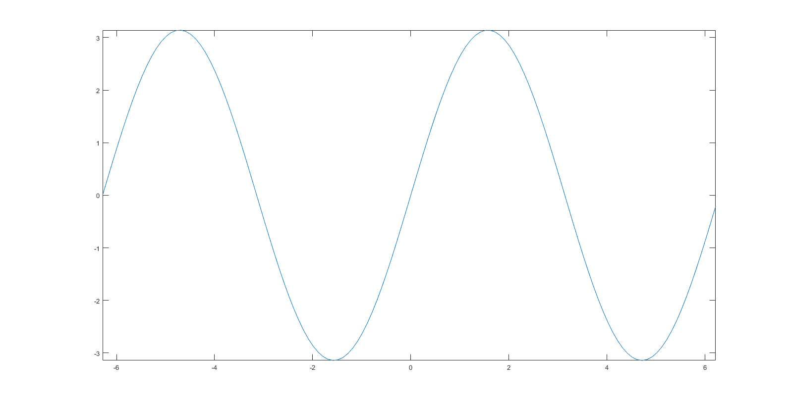
maximize figure

clear; close all; clc;
figure(10);
x = -2*pi:.1:2*pi;
plot(x,pi*sin(x)); axis tight
set(10, 'Position', get(0,'ScreenSize'));
%{
    Sometimes, axes tick labels depend on the figure size. For example, it may
    happen that before maximization the ytick labels are 10^0 and 10^{-5}, while
    they become 10^0, 10^{-2}, 10^{-4}, 10^{-6} after maximization. Note that,
    for this example, saving either the maximized or un-maximized figure, the
    ytick labels remain to be 10^0 and 10^{-5}. On the other hand, if one saves
    the maximized figure manuanlly, then the labels would be 10^0, 10^{-2},
    10^{-4}, 10^{-6}. However, manually saving causes difficulty in scale
    setting in latex
%}

legend items organization

%{
    clear; close all; clc;
    x1 = -pi/2:0.1:pi/2;
    y1 = sin(x1);
    x2 = 0:0.1:pi;
    y2 = cos(x2);
    u = -1:0.1:1;
    v1 = asin(u);
    v2 = acos(u);
    z = -pi/2:0.1:pi;
    Lz = length(z);

    plot_1 = ...
    plot(x1,y1,'r-', ...
        x2,y2,'g-', ...
        u,v1,'b-', ...
        'linewidth',2);
    hold on;

    plot_2 = ...
    plot(u,v2,'k-', ...
        z,zeros(Lz,1),'m-', ...
        zeros(Lz,1),z,'c-', ...
        'linewidth',2);
    hold off;

    legend_plot_x = legend('$\sin(x)$','$\cos(x)$','$\arcsin(x)$');
    set(legend_plot_x,'orientation','horizontal','interpreter','latex','Location','best');

    copyobj(legend_plot_x,gcf);
    legend_plot_y = legend('$\arccos(x)$','$y=0$','$x=0$');
    set(legend_plot_y,'orientation','horizontal','interpreter','latex','Location','best');

    legend_str{1} = '$\sin(x)$';
    legend_str{2} = '$\cos(x)$';
    legend_str{3} = '$\arcsin(x)$';
    legend_str{4} = '$\arccos(x)$';
    legend_str{5} = '$y=0$';
    legend_str{6} = '$x=0$';
    hh = columnlegend(3,legend_str,'Location','NorthWest','boxon');
    set(hh,'interpreter','latex');


    legend('boxoff')
    grid on;
    axis equal tight
%}

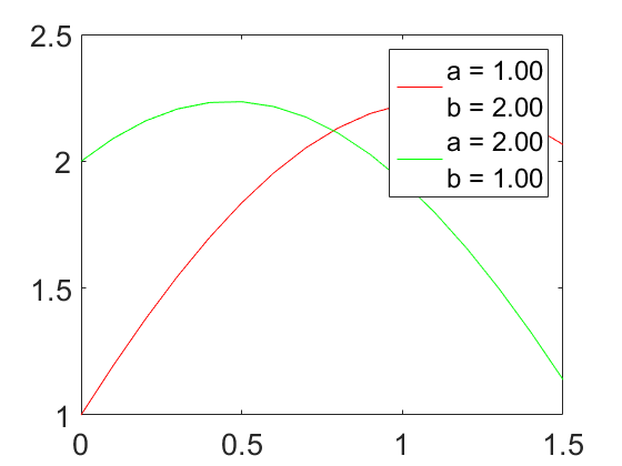
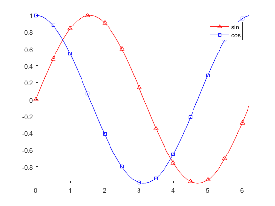
legend: multiple lines in one legend item

clear; close all; clc;
figure(1);
% f = a*cos(x) + b*sin(x);
x = 0:0.1:pi/2;
a1 = 1; b1 = 2;
a2 = 2; b2 = 1;

f = @(a,b,x) a*cos(x) + b*sin(x);
y1 = f(a1,b1,x);
y2 = f(a2,b2,x);

s1 = sprintf( 'a = %0.2f\nb = %0.2f',a1,b1);
s2 = sprintf( 'a = %0.2f\nb = %0.2f',a2,b2);

plot(x,y1,'r-',x,y2,'g-');
legend(s1,s2);
set(gca,'fontsize',20);

legend: multiple legend boxes

%{
    clear; close all; clc;
    t = 0:0.1:2*pi;
    x = cos(t);
    y = sin(t);

    plot_x = plot(t,x,'r-'); hold on
    plot_y = plot(t,y,'g-'); hold off

    [legend_x,~,~,~] = legend(plot_x,'$\cos(t)$',1);
    set(legend_x,'interpreter','latex','fontsize',20);
    copyobj(legend_x,gcf);
    [legend_y,~,~,~] = legend(plot_y,'$\sin(t)$',2);
    set(legend_y,'interpreter','latex','fontsize',20);
    axis tight;
%}

legend: dense data with sparse marker

combine line and marker into one legend item

clear; close all; clc;
t = 0:0.1:2*pi;
x = sin(t);
y = cos(t);
line(t,x,'color','red');
line(t,y,'color','blue');
line(t(1:5:end),x(1:5:end),'linestyle','none','marker','^','color','red');
line(t(1:5:end),y(1:5:end),'linestyle','none','marker','s','color','blue');
[~,oh] = legend('sin','cos');
set(oh(4),'marker','^');
set(oh(6),'marker','s');
axis tight;

legend: dense data with sparse marker

clear; close all; clc; cla;
t = (0:100)/50*pi;
x = sin([1;2;3]*t);
line(t,x);
line(t(1:5:end),x(:,1:5:end),'linestyle','none','marker','^');
[~,oh] = legend('line 1','line 2','line 3');
set(oh(5:2:end),'marker','^');
%{
     How to use different markers with different colors?
 %}

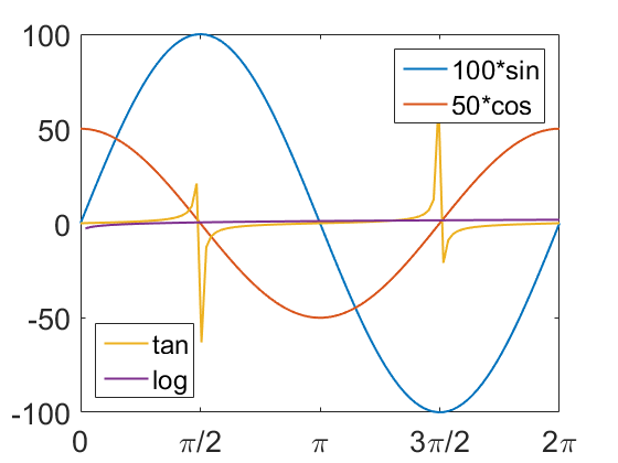
legend(ah,p(3:4)) ??

clear; close all; clc;
figure(1); % axes('fontsize',20);
a = linspace(0,2*pi,100);
y1 = 100*sin(a);
y2 = 50*cos(a);
y3 = tan(a);
y4 = log(a);
y = [y1;y2;y3;y4];
p = plot(a,y,'linewidth',1.5);
% axis tight;
set(gca,'fontsize',20);
set(gca, ...
    'xlim',[0 2*pi], ...
    'xtick',0:pi/2:2*pi, ...
    'xticklabel',{'0' '\pi/2' '\pi' '3\pi/2','2\pi'}, ...
    'ylim',[-100 100], ...
    'ytick',-100:50:100, ...
    'yticklabel',{'-100' '-50' '0' '50' '100'});
legend(p(1:2),'100*sin','50*cos');
ah = axes('position',get(gca,'position'),'visible','off');
legend(ah,p(3:4),'tan','log','location','southwest');
set(gca,'fontsize',20);

legend: columnlegend.m

http://www.mathworks.com/matlabcentral/fileexchange/27389-columnlegend

close all; clear; clc;
x = -2*pi:0.1:2*pi;
y = sin(x); y = y';
Y = repmat(1:10,length(x),1) .* repmat(y,1,10);
plot(Y);
legend_str = cell(10,1);
for i = 1:10
    legend_str{i} = ['str ',num2str(i)];
end
columnlegend(2,legend_str,'Location','NorthEast','boxon','boxoff');

legend: gridLegend.m

%{
    http://www.mathworks.com/matlabcentral/fileexchange/29248-gridlegend-a-multi-column-format-for-legends
    clear; close all; clc;
    gridDemo;
%}

manipulate figure positions

clear; close all; clc;
figure(1);  set(gca,'fontsize',20); set(gcf,'Position',[900,40,400,250]);
semilogy(rand(1000,1),'b-.','linewidth',3);
legend('LADMM','Location','NorthEast');
xlabel('Iteration.'); ylabel('Error in L.'); axis tight;

returns of legend, figure, axis, axes, etc

gcf, gca, etc

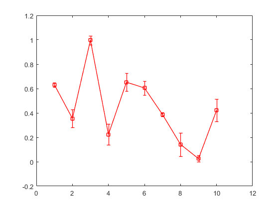
errorbar

clear; close all; clc;
figure(1);
x = 1:10;
d_mean = rand(10,1);
d_std = rand(10,1)*0.1;
errorbar(x,d_mean,d_std,'-rs','linewidth',1);

save data

clear; close all; clc;
foldername = 'matlab_tricks';
filename = 'filename';
data.a = 1; data.b = 2;
save([foldername,'\',filename,'.mat'],'-struct','data');
v1 = 1; v2 = 2; v3 = 3;
save([foldername,'\',filename,'.mat'],'v1','v2','v3');

save in eps, pdf, jpg formats (print)

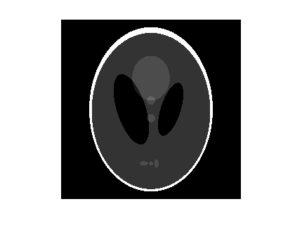
clear; close all; clc;
I = phantom(256);
imshow(I,[]);
foldername = 'matlab_tricks';
filename = 'filename';
saveas(1,[foldername,'\',filename,'.eps'],'psc2');
eval(['print -dpdf ',foldername,'\',filename,'.eps']);
eval(['print -dpdf ',foldername,'\',filename,'.pdf']);

read & write

rgn setting

%{
    SCURR = rng; % keep current rng info in SCURR
    save('filename.mat','SCURR'); % save rng info into a mat file
    load filename.mat; rng(SCURR);
%}

diary

clear; close all; clc;
foldername = 'matlab_tricks';
eval(['diary ',foldername,'one_run_alpha','.txt']);

fopen, fclose

%{
    fopen('rpca_cvx.txt','a+');
    diary rpca_cvx.txt
    diary off;
    fclose('all');
%}

set path, startup path

pathdef.m

eval, mkdir, copy, paste, delete, etc.

make a folder, delete a folder

make a file (with extension), delete a file

%{
    what, cd, dir, addpath, rmpath, genpath, pathtool, savepath, rehash.
    cd, copyfile, delete, dir, fileattrib, movefile, rmdir.
%}

mkdir, eval

current_path = cd;
eval(['!mkdir ' current_path '\subfolder_1']);
eval(['!mkdir ' current_path '\subfolder_2']);

%{
if ~exist(foldername,'dir'), mkdir(foldername); end
    eval(['!del ' defname]);
    eval(['load ' defname]);
    eval(['!copy ' MATNAME ' ' LIPSOLPATH '\tmp\default.mat']);
    filename = [write_folder,'\','cgs_vs_iter_aver_of_12','.',file_format];
    eval(['print -dpdf ',filename]);
    load([foldername,data_filename,'.mat']);
%}

子目录或文件 C:\Users\jy\Desktop\main\codes\matlab_learning\subfolder_1 已经存在。 
子目录或文件 C:\Users\jy\Desktop\main\codes\matlab_learning\subfolder_2 已经存在。

fopen, fclose, fwrite

text

clear; close all; clc;
x = 0:pi/20:2*pi;
plot(x,sin(x));
text(pi,0,' \leftarrow sin(\pi)','FontSize',18);
text(pi,0.5,'\ite^{i\omega\tau} = cos(\omega\tau) + i sin(\omega\tau)',  'fontsize',30);
text(2*pi,0, '$\frac{\|x\|}{\|y\|}$','HorizontalAlignment','Right','interpreter', 'latex','fontsize',30);
%{
    set(0,'DefaulttextProperty',PropertyValue);
    set(gcf,'DefaulttextProperty',PropertyValue);
    set(gca,'DefaulttextProperty',PropertyValue);
    http://www.mathworks.com/matlabcentral/answers/102053-how-can-i-make-the-xtick-and-ytick-labels-of-my-axes-utilize-the-latex-fonts-in-matlab-8-1-r2013a
%}
clear; close all; clc;
x = -pi:0.1:pi;
y = sin(x);
plot(x,y);

% remove ticklabels
set(gca,'xticklabel',[]); % Remove xtick labels
set(gca,'yticklabel', []) % Remove ytick labels

% Get tick mark positions
yTicks = get(gca,'ytick');
xTicks = get(gca, 'xtick');

% Reset the ytick labels in desired font
ax = axis; % Get left most x-position
HorizontalOffset = 0.1;
for i = 1:length(yTicks)
% Create text box and set appropriate properties
     text(ax(1) - HorizontalOffset, yTicks(i), ... % position
         ['$' num2str( yTicks(i)) '$'], ...  % label (in latex format)
         'HorizontalAlignment','Right', ...
         'interpreter', 'latex');
end

% Reset the xtick labels in desired font
minY = min(yTicks);
verticalOffset = 0.1;
for j = 1:length(xTicks)
% Create text box and set appropriate properties
     text(xTicks(j), minY - verticalOffset, ... % position
         ['$' num2str( xTicks(j)) '$'], ... % label
         'HorizontalAlignment','Right', ...
         'interpreter', 'latex');
end
title('tick labels generated by "text"');

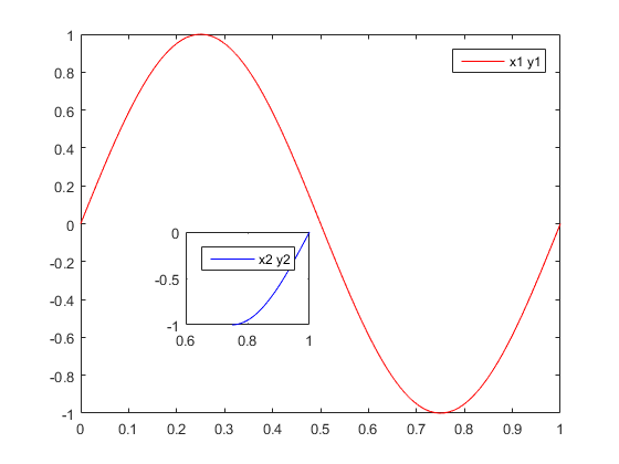
small figure in big: example 1

clear; close all; clc;
x1 = linspace(0,1);
x2 = linspace(3/4,1);
y1 = sin(2*pi*x1);
y2 = sin(2*pi*x2);

figure(1)
% plot on large axes
plot(x1,y1,'r-');
legend('x1 y1');

% create smaller axes in top right, and plot on it
pos.h = 0.3; % horizontal
pos.v = 0.3; % vertical (pos = position)
size.width = 0.2;
size.height = 0.2;
axes('Position',[pos.h,pos.v,size.width,size.height]);
box on
plot(x2,y2,'b-');
legend('x2 y2');

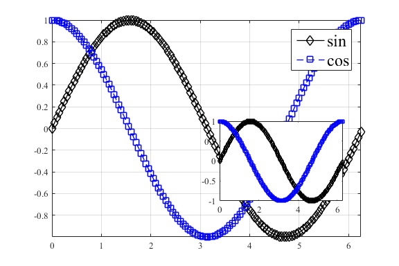
small figure in big: example 2

clear; close all; clc;

TextFontSize = 20;
LegendFontSize = 18;

set(0,'DefaultAxesFontName','Times',...
    'DefaultLineLineWidth',1,...
    'DefaultLineMarkerSize',8);
set(gca,'FontName','Times New Roman','FontSize',TextFontSize);
set(gcf,'Units','inches','Position',[0 0 6.0 4.0]);

x = 0:0.05:2*pi;
y = sin(x);
z = cos(x);
plot(x,y,'-dk')
hold on
plot(x,z, '--sb')
hold on
grid on
axis tight
hg1 = legend('sin','cos',1);
set(hg1,'FontSize',LegendFontSize);

set(0,'DefaultTextFontName','Times',...
    'DefaultAxesFontName','Times',...
    'DefaultLineLineWidth',1,...
    'DefaultLineMarkerSize',4.5);

% set the position and the size of the small figure
h1 = axes('position',[0.55 0.245 0.31 0.3]);
set(h1,'FontName','Times New Roman','FontSize',16);
axis(h1);
plot(x,y,'-dk');
hold on
plot(x,z,'--sb');
hold on
xlim([0 2*pi]);
ylim([-1,1]);

make a vedio

%{
    clear; close all; clc;
    aviobj = avifile('Fenchel.avi');
    for ii = 1:count
        h = imagesc(imread([num2str(ii),'.jpg']));
        %h = imread([num2str(ii),'.jpg']);
        frame = getframe(gca);
        aviobj = addframe(aviobj,frame);
    end
    aviobj = close(aviobj);
%}

%{
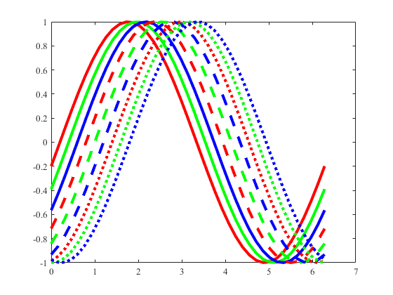
    clear; close all; clc;

    x = -pi:pi/20:pi;
    sin_nx = @(n,x) sin(n*x);
    cos_nx = @(n,x) cos(n*x);
    y1 = sin_nx(1,x);
    y2 = sin_nx(3,x);
    y3 = cos_nx(1,x);
    y4 = cos_nx(3,x);

    figure(1);
    % set(0,'DefaultAxesLineStyleOrder',{'-',':','--','-.'});
    set(1,'LineStyleOrder',{'-',':','--','-.'})
    p1 = plot(x,y1); hold on;
    p2 = plot(x,y2);%,x,y3,x,y4);
    % legend('r-','b:','k--','m-.',0);

    set(p1,'Color','r','LineWidth',2)
    set(p2,'Color','g','LineWidth',2)
%}

%{
Line style specifiers: '-','--',':','-.','none'

Marker specifiers:
 '+','o','*','.','x','s','d','^','v','>','<','p','h','none'

Color specifiers: r, g, b, c, m, y, k, w
%}

groot: Graphics root object - MATLAB groot - MathWorks (starting from 2014b)

clear; close all; clc;

set(0,'defaultAxesColorOrder',[1 0 0;0 1 0;0 0 1],...
      'defaultAxesLineStyleOrder','-|--|:')


t = 0:pi/20:2*pi;
a = ones(length(t),9);
for i = 1:9
    a(:,i) = sin(t-i/5)';
end
plot(t,a,'linewidth',3);
%{
    set(groot,'defaultAxesLineStyleOrder','remove')
    set(groot,'defaultAxesColorOrder','remove')
%}

delete white margin

clear; close all; clc;
n = 256;
I = zeros(n);
r = [128 64 192];
c = [20 200 200];
J = roipoly(I,r,c);

figure(1);
% h = imshow(J,'border','tight','initialmagnification','fit');
% set(gcf,'Position',[0,0,500,500]);
% axis normal;
imshow(J,[]);

folder = 'matlab_tricks/';
filename = 'no_white_margin';
print('-depsc',[folder,filename]);
input_file = [folder,filename,'.eps'];
input_file_content = fileread(input_file);
output_file = fopen(input_file, 'wt');
fwrite(output_file, input_file_content);
fclose(output_file);
system(['epstopdf ' input_file]);

done

close all;
disp('done');

done

Contents

(xticklabel, yticklabel, latex): an example

latex interpreter

maximize figure

legend items organization

legend: multiple lines in one legend item

legend: multiple legend boxes

legend: dense data with sparse marker

legend: dense data with sparse marker

legend(ah,p(3:4)) ??

legend: columnlegend.m

legend: gridLegend.m

manipulate figure positions

returns of legend, figure, axis, axes, etc

gcf, gca, etc

errorbar

save data

save in eps, pdf, jpg formats (print)

read & write

rgn setting

diary

fopen, fclose

set path, startup path

eval, mkdir, copy, paste, delete, etc.

make a folder, delete a folder

make a file (with extension), delete a file

mkdir, eval

fopen, fclose, fwrite

text

small figure in big: example 1

small figure in big: example 2

make a vedio

groot: Graphics root object - MATLAB groot - MathWorks (starting from 2014b)

delete white margin

done